Objective 1: Describe the wave nature of electromagnetic radiation and list the various types of electromagnetic radiation by wavelength and frequency.
It may seem weird to start with a discussion of electromagnetic radiation, waves, and frequency when looking at chemistry and electrons. Why do this? This topic is titled “electronic structure of atoms”. Electronic structure of atoms turns out to be a description of where the electrons are found (or at least likely to be found) in an atom, as well as the kinetic and potential energy of these electrons. Much of what is known about the electronic structure of atoms was obtained by observing the interaction of how light (one form of electromagnetic radiation) interacts with matter.
Electromagnetic radiation and waves
Electromagnetic radiation carries energy through space. There are many forms of electromagnetic radiation that are familiar – including visible light, radio waves, x-rays, microwaves, and others.
All of the forms move through a vacuum at a speed of 3.00X10⁸ meters per second , commonly called the”speed of light”: The speed of light is symbolized by c:
c=3.00 X 10⁸ m/s
Why it it called electromagnetic radiation? The term electromagnetic comes from the fact that the radiation is an oscillating electric field perpendicular to an oscillating magnetic field. These oscillating fields are described as waves. Even though there are two waves perpendicular to each other, we often illustrate it by drawing just one (the second is similar, but would be coming out of and into the paper if the first were drawn on the paper).
Characteristics of waves
Figure 6.2 in OpenStax illustrates a drawing of a wave:
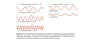
As you look at the left side of Figure 6.2, you see three waves. As you look from top to bottom, the wavelength gets shorter. Wavelength is the distance from peak to peak (or trough to trough). The units are distance units (m, km, nm, etc) The symbol for wavelength is the Greek letter lambda (λ) .
λ=wavelength
As the wavelength gets shorter, the frequency gets higher (higher frequency means more repetitions or cycles of the wave in a given time). The frequency of a wave is the number of complete wavelengths or cycles that pass a given point each second. As you look at the three waves on the left of Figure 6.2, the frequency gets higher as you go down. The symbol is the Greek letter nu (ν). The common for frequency is Hertz (Hz) where 1 Hz is 1 cycle/second or 1/s or s-1. Metric frequencies are used with Hertz, radio frequencies are often in megahertz (MHz) or kilohertz (kHz), for example.
Frequency and wavelength are inversely proportional. The longer the wavelength, the lower the frequency. The shorter the wavelength, the higher the frequency.
The waves on the right of Figure 6.2 illustrate amplitude. The one on the top has higher amplitude than the one on the bottom. Amplitude is the distance from node to crest or trough (height of the wave). Amplitude is related to intensity of the wave – a larger amplitude light wave would correspond to brighter light.
Types of Electromagnetic Radiation
The type or form of radiation depends on its wavelength (or frequency). Figure6.3 in OpenStax illustrates different forms of electromagnetic radiation depending on wavelength.
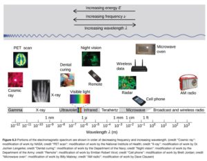
I would not expect you to state the type of radiation of given a numerical wavelength, but you should be familiar of the “order” of different types of radiation with respect to increasing or decreasing wavelength, frequency, or energy (we haven’t talked about energy yet, but energy is directly proportional to frequency – energy increases proportionally as frequency gets higher).
The types of radiation are listed below in order of increasing frequency, increasing energy, and decreasing wavelength:
- Radio
- Microwaves
- Light
- Infrared
- Visible
- Red
- Orange
- Yellow
- Green
- Blue
- Indigo
- Violet
- Ultraviolet
- X ray
- Gamma Ray
Objective 2: Knowing the speed of light, convert between wavelength and frequency of electromagnetic radiation.
The relationship between wavelength and frequency
Where
- c = 3.00 X 10⁸ m/s (the speed of electromagnetic radiation in a vacuum)
- λ is wavelength
- ν is frequency.
Since c is a constant, if you know the wavelength you can calculate the frequency and vice-versa. If you use 3.00 X 10⁸ m/s for c, then wavelength will be in meters and frequency will be in s-1 or Hz.
Objective 2 Example
Electromagnetic radiation with a wavelength of 532 nm is green light. Calculate its frequency in hertz.


Since c = 3.00 X 10⁸ m/s, we need λ in m

and

Objective 2 Practice
Photosynthesis uses light with a frequency of 4.54 x 10¹⁴ s-1. What wavelength does this correspond to in nm?
Objective 3: Describe the essential features of Planck’s quantum theory and interconvert among wavelength, frequency and energy of a quantum.
Quantization of Energy
Max Planck, when studying electromagnetic radiation emitted from solids heated to very high temperatures, found electromagnetic energy to be quantized. “Quantized” means that one can only have certain amounts. As an example, the number of children in a family is quantized – there can only be certain amounts (1,2,3,4…). A family cannot have 1.8, 4.5, 2,4356, or 3.00446 kids!
Similarly, Planck found that electromagnetic energy could only be emitted by atoms in certain “bundles” or amounts. The “bundle” of energy is called a quantum. The amounts of energy that could be emitted were 1 quantum, 2 quanta (the plural of quantum), 3 quanta, 4 quanta,……very large (whole) numbers of quanta.
How much energy does a quantum contain? It turns out that that depends on the frequency. Higher frequency light has more energy/quantum than lower frequency (see Figure 6.3 in OpenStax) In fact, energy and frequency are directly proportional and related by the equation:
Where:
- E is the energy of the quantum in J
- h=6.626 X 10⁻³⁴ J·s (h is known as Planck’s constant)
- ν is frequency in s-1.
Objective 3 Example
Calculate the energy of a quantum of green light with a wavelength of 532 nm.
We can use the equation 

Solving for energy,

A quantum of radiation with a wavelength of 532 nm is 3.73 X 10⁻¹⁹ J. Therefore, energies of radiation with this wavelength must be:
3.73 X 10⁻¹⁹ J, 2(3.73 X 10⁻¹⁹) J, 3(3.73 X 10⁻¹⁹) J……
For a more in-depth discussion of this, read “the section “Blackbody Radiation and the Ultraviolet Catastrophe” in OpenStax section 6.1.
Objective 3 Practice
Photons
As a result of Einstein’s work on the photoelectric effect (see Figure 6.11 OpenStax and read the surrounding section titled Photoelectric Effect), Einstein determined that since energy from electromagnetic energy is quantized, the radiation itself behaved as if it were a stream of particles (each with the energy of one quantum)- called photons.
The energy of a photon is the energy of a quantum

Another useful equation combines
Objective 4: Using the de Broglie equation, calculate particle wavelength given particle mass and velocity.
For many years, scientists had a very good understanding of the behavior of light and electromagnetic radiation as a wave. Using the known properties of waves, they were able to explain the behavior of light and design optics including telescopes, glasses, etc. But the quantization of energy demonstrated that electromagnetic radiation, which has properties of waves, acts like a particle too. These particles are called photons.
DeBroglie proposed that if light, which was long thought of as a wave, also acts like a small moving solid object or particle (photons), then maybe matter, which is particles, also acts as a wave. He determined that the wavelength of a moving particle (called the De Broglie wavelength (λ) could be calculated by this equation:

Where
- h= Planck’s constant
- m is the mass of the particle in kg
- v is velocity in m/s (not frequency).
So a solid object in motion, for example a baseball flying through the air, is also a wave. This is an example of particle wave duality. Particle wave duality is the idea that radiation, which was always understood to be waves, has particle properties (shown by quantization) while particles also have wave properties (shown by the DeBroglie wavelength).
Objective 4 example
Calculate the wavelength of a 145 g baseball traveling 100. mph (44.5 m/sec)
Recall, the mass has to be in kg. Therefore, 0.145 kg rather than 145 g is used. Why kg? Because using SI Units for all the parameters will allow the units to cancel properly, and joules (the J in the J⋅s unit for Planck’s constant, is in SI units. We can think of SI units as a ststem of units designed to work together and cancel. If h, m, and v are all in SI units, then the units for wavelength will be in the SI unit for distance, which is the meter. So the problem and units will work like this:

If you prefer to see the units cancel, you have to realize that

Then the problem can be written as:

Either way, the resulting wavelength of the baseball is very, very small (1.02 X 10⁻³⁴ m), especially compared to the size of the baseball. It is so small that we can neglect the wave properties of the baseball entirely and still perfectly understand and describe its motion using particle (classical) mechanics as Isaac Newton did. On the other hand, the wavelength of a photon is so large compared to the photon that describing light as a wave worked perfectly well for hundreds of years. Electrons, though, are weird. It turns out that they are large enough that we must consider their particulate behavior but small enough that we must also consider their wave behavior to adequately describe their motion and behavior in an atom. More on that later.
De Broglie Wavelengths
| Object (Particle) | Mass (kg) | Wavelength (m) | Acts like* |
| Photon – green visible light | 4.15 X 10-36 | 5.32 X 10⁻⁷ | Wave |
| Electron | 9.11 X 10⁻³¹ | 7.27 X 10⁻¹¹** | Both particle and wave |
| Baseball | 0.145 | 1.02 X 10⁻³⁴ | particle |
*All matter has both particulate and wave properties.
We can largely ignore the particle properties of light and still describe its behavior.
We can largely ignore the wave properties of a baseball and still describe its behavior.
** DeBroglie wavelengths are more often calculated for particles like electrons. The wavelength of an electron from the Table is calculated in Example 6.6 in OpenStax Section 6.3.
Objective 5: Explain the origin of the line spectra.
Atomic Emission Spectra
Samples of elements can be hit with energy using an energy source. The elements absorb the energy. They then release the energy as electromagnetic radiation (emission). Dispersion of emitted radiation into its wavelengths produces a spectrum. If the spectrum contains all wavelengths, it is called a continuous spectrum. A rainbow is an example of a continuous spectrum. If the spectrum only contains only certain specific wavelengths, it is called a line spectrum (as the specific wavelengths show up as lines (see Figure 6.13 OpenStax)
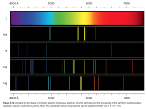
The radiation emitted by excited gaseous atoms form a line spectrum. The line spectrum, which showed that atoms could only emit certain wavelengths of radiation, also means that the atom can only emit certain energies as radiation, as

The Bohr Model of the atom took these results and attempted to explain then with a new model of the atom.
Objective 6: Describe the Bohr model of the hydrogen atom.
The Bohr Model of the atom (1913) explained the line spectrum of hydrogen. An overview of the model is presented here. It is discussed in more detail in OpenStax Section 6.2.
In the model, the electrons go around the nucleus in elliptical orbits. Any electrons in higher energy levels orbit further from the nucleus. Electrons in the lower orbits are more closely bound to the nucleus. When an electron descends from a higher energy (outer) orbit to a lower energy (inner) orbit, energy corresponding to the difference in the energy of the two levels is released. It is released as a photon of a certain frequency ν or wavelength λ as calculated by
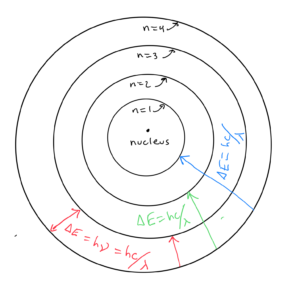
An electron going from level n=4 to n=3 would emit a photon of a wavelength or frequency corresponding to the energy difference between n=4 and n=3. Since an electron going from level n=4 to n=1 would have a bigger energy difference ΔE, it would emit a photon of higher frequency or shorter wavelength, as calculated by 
Energy Levels and the Bohr Model
Bohr calculated the energies corresponding to each allowed orbit for the electron in the hydrogen atom. The lowest energy orbit, called the ground state, is assigned a value of n=1. Higher energy orbits are n=2,3,4, etc. The energy of an electron in each orbit is given by:
The resulting energies are shown in OpenStax Figure 5.14. For example, for n=3

As n →∞, E → 0. The energy of each energy level is negative, and the lower the energy level, the more negative the energy.
How the Bohr Model is correct
It calculates the correct energy for energy levels of hydrogen, and it calculates the correct wavelengths (or frequencies) for the atomic spectrum of hydrogen. It also explained that the electron’s energies are quantized.
How the Bohr Model is incorrect
The electrons do not circle the nucleus in elliptical orbits. The Bohr model gives the incorrect physical picture as it did not take into account the wave nature of electrons. Also, the calculated energies are incorrect for all elements other than hydrogen, as the Bohr model does not account for how the electrons affect each other.
Objective 7: Calculate the energy difference between any two electronic states of a hydrogen atom and the wavelength or frequency of the photon involved in the transition.
A transition is defined as an instance when an electron goes from one orbit in the Bohr model to another. Energy is required for the electron to go from a lower to a higher level. The energy is supplied by an absorbed photon, whose frequency or wavelength can be calculated by
Energy is released when the electron goes from a higher to lower level. The energy is released as an emitted photon, whose frequency or wavelength can be calculated by
How are the energies calculated? The energy of an electron at an allowed energy level n of a hydrogen atom is calculated by the equation 
Objective 7 example:
Calculate the energy change which occurs when an electron in a hydrogen atom Bohr orbit n= 2 drops to the ground state.
The ground state is the n=1 level. Therefore, the energy difference will be:

Objective 7 Practice:
Calculate the wavelength of the photon associated with the relaxation of an electron from the n=3 to the n=1 energy level of the hydrogen atom Is the photon absorbed or emitted?
Objective 8: Explain the significance of the wave function and the square of the wave function of an electron as they pertain to the orbital, electron density and probability.
The currently accepted explanation of where the electrons are in the atom is provided by quantum mechanics, which takes into account both the particle and wave behavior of the electron. Schrodinger treated the electron as a wave, and used the known physics and math for standing waves in developing the Schrodinger Equation, which can be solved to describe the electron’s behavior:

Where
(the Hamiltonian operator) is a set of mathematical instructions accounting for the potential energy of attraction between the nucleus and the electron and the kinetic energy of electron motion.
(the wavefunction) is a function or equation that is a solution of the Schrodinger equation. Several wavefunctions are correct solutions of the Schrodinger equation.
- E (energy) is the total kinetic and potential energy of the electron in the atom
The Schrodinger equation looks simple, but it is not. We cannot cancel the
Similarly, B(4)=43, and B(50)=503. We could also apply B to an equation:
B(3x + 2y + 5) = (30x + 20y + 50)+3 = 30x + 20y + 53
That’s what 
Why use
It turns out that when you do 
Objective 9: Describe the Heisenberg uncertainty principle.
Why do we have to deal with “probabilities” of where the electron is in the atom instead of just knowing where it is? The Heisenberg Uncertainty Principle states that we cannot precisely know the position and momentum of a particle at the same time. The principle applies to all moving objects. Uncertainty is very small compared to everyday objects we can see, so it is inconsequential for these large objects. However, the uncertainty is significant with very small particles (like electrons). The principle is explained mathematically and in more detail in OpenStax Section 6.3.
Momentum is defined as mass times velocity. Velocity is speed in a certain direction. Since the mass of an electron is known, we cannot know both the location of the electron in the atom and its velocity. In other words, we can’t know where the electron is around the atom and know where it is going. Instead, we must deal with probabilities.
The square of the wavefunction gives the probability of finding the electron in a certain location. Plots of the square of the wavefunction ,
Objective 10: Explain the physical significance of each quantum number and know the restrictions on possible values.
In the last objectives, we saw that orbitals describe where an electron is most likely to be found in an atom, and that they are plots of wavefunctions, which are themselves equations. Wavefunctions are complicated equations, so instead of writing them out it is customary to describe them with three numbers called quantum numbers.
While the idea of describing equations with numbers might sound weird to you, it is something you are familiar with– if I asked you to draw a line with a slope of 2 and a y-intercept of 3, you could do it, as well as write the equation:
slope = m = 2
y-intercept = b = 3
Equation: y=mx+b or y=2x+3.
Just as two numbers (m and b) can describe a line (which can be plotted), three numbers (the quantum numbers n,l, and ml) can describe an orbital, which can be plotted. The three quantum numbers (and their rules, as they can only have certain values, are discussed next.
The quantum number n (Principal Quantum Number)
What it tells us: Orbital energy and size
Allowed numbers: Whole positive numbers, starting with 1. (1,2,3,4…..)
How it works: The larger the value of n, the higher the probability the electron is further from the nucleus. Therefore the orbital is larger. Also, the larger n, the higher energy the electron. The energy agrees with that calculated by the equation used for the energies for levels n=1,2,3,4… in the Bohr model.
The quantum number l (Angular Momentum Quantum Number)
What it tells us: Orbital shape (the shapes corresponding to each number l are shown in OpenStax Figure 6.21)
Allowed numbers: 0,1,2,3,4 etc to a maximum of n-1
How it works: The possible values for l depend on the value of n.
- If n=1, l can only be 0.
- If n=2, l can be 0 or 1.
- If n=3, l can be 0, 1, or 2.
- If n=4, l can be 0, 1, 2, or 3.
- If n=12, l can be 0, 1, 2, 3, 4, 5, 6, 7, 8, 9, 10 ,or 11.
- and so on
The quantum number l also gives us the orbital “letter name”:
- l=0: s orbital
- l=1: p orbital
- l=2: d orbital
- l=3: f orbital
- l=4: g orbital
- l=5: h orbital
- and so on, though we will not go beyond f
Orbitals are often labeled by a “designation” which is defined by their n and l numbers, using the “letter name” for l.
- If n=1, l = 0: 1s
- If n=2, l =0: 2s
- If n=2, l =1: 2p
- If n=3, l =1: 3p
- If n=5, l=2: 5d
The quantum number ml (Magnetic Quantum Number)
What it tells us: Orbital orientation in space (direction it faces)
Allowed numbers: whole numbers with a minimum of – l and a maximum of +l
How it works: The possible values for ml depend on the value of l.
- If l=0, ml can only be 0. (there can be one s orbital for a given value of n)
- If l=1, ml can be -1, 0, or +1. (there can be three p orbitals for a given value of n)
- If l=2, ml can be -2, -1, 0, +1, or +2. (there can be five d orbitals for a given value of n)
- If l=3, ml can be -3, -2, -1, 0, +1, +2, or +3. (there can be seven orbitals for a given value of n)
Example of how it all fits:
Let’s look at the possibilities if n=3 and l=1.
- These orbitals are called 3p orbitals
- All three of them have the quantum numbers n=3 and l=1.
- Each of the three has its own value of ml (one is -1, one is 0, and one is +1).
Similarly, there would be three 2p orbitals (or seven 4f orbitals)
Electron Shells and Subshells
The collection of orbitals with the same value of n are called an electron shell. Orbitals that have the same n and l value are called a subshell. Each subshell is designated by a number (the value of the quantum number n) and a letter s, p, d, or f (determined by the value of the quantum number l ). The shell with a value of n will consist of exactly n subshells. An s subshell consists of 1 orbital, p has 3, d has 5 and f has 7 orbitals. Finally, the total number of orbitals in a shell “n” is n2
Electron Shells and Subshells – example
The above information on shells and subshells is somewhat abstract on its own — it is often easier to see with an example, so we will look at it in light of the n=3 shell.
The collection of orbitals with the same value of n are called an electron shell. For this example, lets consider the n=3 shell.
Orbitals that have the same n and l value are called a subshell. Each subshell is designated by a number (the value of n) and a letter s, p, d, or f (value of l )
For n=3, l can be 0,1,or 2
- The orbitals with n = 3 and l = 0 are in the 3s subshell
- The orbitals with n = 3 and l = 1 are in the 3p subshell
- The orbitals with n = 3 and l = 2 are in the 3d subshell
The shell with a value of n will consist of exactly n subshells. For n=3, there are 3 subshells: 3s, 3p, 3d.
s subshell consists of 1 orbital, p has 3, d has 5 and f has 7 orbitals.
- the 3s subshell has 1 orbital, with ml=0
- the 3p subshell has 3 orbitals, with ml=-1, 0, and +1
- the 3d subshell has 5 orbitals, with ml=-2, -1, 0, +1, +2
The total number of orbitals in a shell “n” is n2. Note the one 3s, three 3p, and five 3d orbitals give a total of 9, and n2= 32 =9.
Objective 10 practice
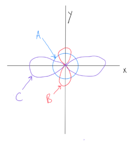
Objective 11: Describe the shapes and orientations in space of the s and p atomic orbitals.
Drawings for s, p, d and f orbitals are in OpenStax Figure 6.21. This interactive link from ChemTube3D shows drawings of the orbitals as well.
s Orbitals
Note from OpenStax Figure 6.21 and ChemTube 3D there is only one shape for s orbitals – spherical (with the nucleus at the center). The radius of the sphere increases with the value of n. Therefore, as you go from 1s to 2s to 3s and so on, the orbitals (spheres) get larger.
p Orbitals
Note from OpenStax Figure 6.21 and ChemTube 3D there is only one shape for p orbitals – there are two lobes going out in opposite directions from the nucleus. One of them is along the x axis (npx), another is along the y axis (npy), and the third is along the z axis (npz). The orbital lobes are sometimes drawn in various shapes (more rounded or more elongated) in order to show a more accurate shape or make for a cleaner drawing. I’m not so concerned about which shape you use as that you understand the two lobes and directions they are facing.
As with s, the orbital size increases with the value of n. Therefore, as you go from 2p to 3p to 4p and so on, the orbitals get larger.
d Orbitals
Note from OpenStax Figure 6.21 and ChemTube 3D there are two shapes for d orbitals – four are shaped the same with four lobes each (but oriented in different directions), and the fifth (with ml = 0) with a unique shape (two lobes with a donut around the middle).
f Orbitals
Note from OpenStax Figure 6.21 and ChemTube 3D that the f orbitals get more complicated still!
Drawing Orbitals
You should be able to sketch the shape of s and p orbitals. Additionally, you should understand the effect the n quantum number has on an orbital — larger n means bigger orbitals, as the electrons in them are higher in energy and have a higher probability of being further from the nucleus. Also, you should be able to differentiate between px, py, and pz
Objective 11 Practice
Objective 12: Use the Aufbau principle, the Pauli exclusion principle and Hund’s rule to predict how electrons will fill orbitals in an atom.
Atoms with more than one electron
All of the orbitals shown above are for atoms with one electron (hydrogen). The quantum mechanical treatment considers the attraction the electron has to the nucleus and its kinetic energy.
But when we consider helium, which has two electrons, now when we look at an electron, in addition to its kinetic energy and attraction to the nucleus, it also faces repulsion from the other electron. This must also be taken into account in solving the Schrodinger equation for the helium electrons.
Anytime an atom has more than one electron, each electron faces repulsion from the other electrons (in addition to attraction to the nucleus and its kinetic energy). This repulsion from other electrons will affect its motion and position in the atom. The problem is that these repulsion forces can’t be calculated exactly since we don’t exactly know where the electrons are and where they are going. Remember, the Heisenberg Uncertainty Principle tells us we cannot know both the position and momentum of an electron, so we can’t know exactly how an electron is repelled by the other electrons.
This means that the Schrodinger equation cannot be solved exactly. Instead, approximate solutions have been found using numerical methods. over the years, these solutions have gotten better and better (as shown by comparsion with spectroscopic experemental results) as computers have gotten more and more powerful. The resulting approximate solutions yield “hydrogenlike” orbitals in atoms with more than one electron. These “hydrogenlike” orbitals are similar in shape to orbitals, but different from hydrogen’s orbitals in size and energy.
Result – orbital energies are different in atoms with more than one electron! Lets look at how they are different.
Orbital energies for atoms with one electron
For a one-electron H atom, orbitals with the same n (principal quantum number) have the same energy. In other words, the 2s and 2p orbitals are equal in energy to each other and higher in energy than the 1s. The 3s,3p, and 3d are equal in energy to each other and higher in energy than the 2s and 2p. Orbitals in the same shell (same n) are called degenerate orbtals, where degenerate means equal in energy.
Orbital energies for atoms with more than one electron
If there is more than one electron, electrons in ns, np, nd, etc subshells experience different repulsions from the other electrons. For example, an electron in a 2s orbital would be affected differently by repulsions from the other electrons than an electron in a 2p orbital. Therefore, in these atoms, orbitals in the same shell are no longer degenerate. In a particular shell, the energy increases as you go from s to p to d to f and so on. The overall resulting ranking of the energies is shown in OpenStax Figure 6.22.
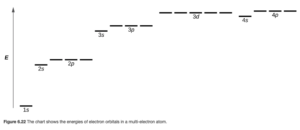
Note from the diagram that the 3d orbitals are so much higher in energy than the 3s that they are also higher than the 4s.
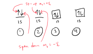
The fourth quantum number: the electron spin quantum number (ms)
As you learned earlier, each orbital is defined by three quantum numbers: n,l, and ml. Each orbital can hold two electrons. The two electrons exhibit the opposite magnetic moment in a magnetic field. This could be explained by the negative charges spinning in opposite directions. This is the basis for the electron spin quantum number (ms). This quantum number can have two possible values:
ms = + ½ or – ½.
If an orbital contains two electrons (its maximum), one of them will have ms = + ½ and the other will have ms = –½.
Electrons with ms = + ½ are sometimes referred to as “spin-up” while electrons with ms = – ½ are referred to as “spin-down”.
As a result, each electron in an atom can be defined by four quantum numbers:
- the first three numbers (n, l, ml ) describe which orbital the electron is in.
- the fourth number (ms) describes its spin (up or down).
The Pauli Exclusion Principle says: no two electrons in an atom can have the same set of four quantum numbers n, l, ml, and ms. Another way to state the Pauli Exclusion Principle it that an orbital can hold a maximum of two electrons and they must have opposite spins.
Objective 12 Practice
Objective 13: Give the electronic configuration of atoms.
A helium atom contains two electrons. What would the 4 quantum numbers be for each of the two electrons, assuming they are in their ground (lowest possible energy) state?
As we can see in OpenStax Figure 6.24, the lowest available energy orbital is the 1s. It can hold up to two electrons, which is all helium has.

Therefore, n=1 and l=0. For l=0, the only value of ml is 0. Since there are two electrons in the orbital, one will have ms=+1/2 and the other will have ms=-1/2.
The quantum numbers of the two electrons will be:
| electron | n | l | ml | ms |
| 1 | 1 | 0 | 0 | +1/2 |
| 2 | 1 | 0 | 0 | -1/2 |
Electron configurations and orbital diagrams are two ways of representing these electrons.
Electron Configurations
The way in which electrons are distributed among the various orbitals of an atom is called the electron configuration of the atom. Atoms normally exist at their lowest energy state (ground state) so the orbitals are filled in order of increasing energy in the order shown in OpenStax Figure 6.24, with no more than two electrons per orbital. The orbitals are given by their subshell designation, and the number of electrons in a subshell is given as a superscript.
The ground state electron configuration for helium would be:
1s2 : this signifies that there are two electrons in the 1s orbital.
Orbital Diagrams
In orbital diagrams, each orbital is shown as a link or a square and each electron in the orbital is shown as an arrow. Arrows pointing up represent spin quantum number ms= + ½ and arrows pointing down represent spin quantum number ms= – ½.
Four ways of drawing the orbital diagram helium would be:
Electron configurations and orbital diagrams are explained very well in OpenStax Section 6.4. If I were to write up notes or videos to explain it, I would pretty much explain it as it is done in this section. I would recommend strongly that you read it and consult it as you practice writing electronic configurations and orbital diagrams. Fron that, you should be able to write an electron configuration or orbital diagram for any element — I will highlight a few aspects or fine points below.
Hund’s rules
Hund’s rules for orbital diagrams come into play when one has a choice on how a set of p, d, or f orbitals are filled for the ground state orbital diagram. The smallest atom this applies to is carbon, which has an electron configuration of 1s22s22p2.
The issue comes down to how the 2 electrons in the 2p orbitals will partially fill the 2p subshell. There are six “slots” for orbitals in the orbital diagram, which means there are 15 different ways those two electrons could go into the 2p orbitals. They are not all equal in energy. Hund’s rules say:
- Electrons will want to stay as far apart as they can, so all the degenerate orbitals will have 1 electron before any have 2. That means all three of the orbitals will get one electron before any of them get two.
- As the electrons fill the orbitals, they will be all spin up (all ms= +1/2) or all spin down (all ms = -1/2) first (unpaired spins) before the second electrons go into orbitals with the opposite spin. Therefore, electrons will fill the 2p subshell either “up, up, up, down, down, down” or “down, down, down, up, up, up”.
As a result, the orbital diagram for carbon will be as follows:
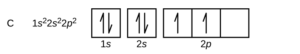
If you examine the orbital diagrams for C,N, and O in OpenStax Section 6.4, you can see how they fill as a result.
Valence electrons and chemical periodicity
Valence electrons are defined as the electron(s) in the outermost shell (highest n quantum number) of an atom. The inner electrons are the core electrons.
Example: Na:
- Electron configuration:
- Core electrons:
- Valence electrons:


Rules for defining valence electrons
- Only electrons in the outer most energy level (highest n quantum number) are valence. In our sodium example above, the 1s,2s, and 2p electrons are core. Only the outermost n quantum number (n=3 in the 3s) is valence.
- For main group (representative) elements (elements in s and p orbitals) electrons in filled d or f shells are not valence electrons.
Example for rule 2:
Br has an electron configuration of:

Only the 4s and 4p (not the 3d) electrons are valence electrons. Therefore Br has 7 (not 17) valence electrons.
Elements in the same column of the periodic table have the same outer (valence) electron configuration. We saw that Na has one valence electron. Li, K,Rb, Cs, and Fr (in the same alkali metal group) also have one valence electron. We saw that Br has 7 valence electrons — the other halogens F,Cl, and I also have seven.
That’s why they behave similarly chemically. Elements with filled shells are particularly stable, making electron configuration a large influence on chemical behavior. This is referred to as the noble gas configuration. Elements with half filled p,d,f etc. subshells are also relatively stable.
Electron configuration of ions
In Unit 1, when learning formulas and nomenclature, you learned that Group I or Alkali Metals such as Li, Na, and K tended to form ions with a +1 charge in ionic compounds. If we look at the electron configuration of Na:
we can see if it loses one electron (the valence 3s) it will, as the Na+ ion, have the same stable noble gas configuration as Ne:
Since these noble gas configurations are so stable, it is relatively easy for Na to lose that electron, making a +1 ion. The same holds for Li, K, and other Group 1 metals.
If we look at Br:
we can see that gaining one electron to form Br –would result in the following electron configuration for Br–:

which is a noble gas configuration.
The oxide (O2–) and sulfide (S2-) ions have a -2 charge because there is a tendency for oxygen and sulfur to gain two electrons to get noble gas configurations like neon and argon.
Condensed electron configurations
Since electron configurations can become long and cumbersome (especially as you go further down the periodic table), and since valence electrons are so important in determining chemical behavior, chemists often write condensed (or shorthand) electron configurations. In these, the previous noble gas is substituted for its electrons in the configuration. Here are some examples:
Br electron configuration:
Br condensed electron configuration:
![[Ar]4{{s}^{2}}3{{d}^{10}}4{{p}^{5}}](https://s0.wp.com/latex.php?latex=%5BAr%5D4%7B%7Bs%7D%5E%7B2%7D%7D3%7B%7Bd%7D%5E%7B10%7D%7D4%7B%7Bp%7D%5E%7B5%7D%7D&bg=ffffff&fg=000&s=0&c=20201002)
P electron configuration:

P condensed electron configuration:
![[Ne]3{{s}^{2}}3{{p}^{3}}4{{s}^{2}}3{{d}^{10}}4{{p}^{5}}](https://s0.wp.com/latex.php?latex=%5BNe%5D3%7B%7Bs%7D%5E%7B2%7D%7D3%7B%7Bp%7D%5E%7B3%7D%7D4%7B%7Bs%7D%5E%7B2%7D%7D3%7B%7Bd%7D%5E%7B10%7D%7D4%7B%7Bp%7D%5E%7B5%7D%7D&bg=ffffff&fg=000&s=0&c=20201002)
Copper and chromium (and the elements below them) are exceptions to ground state configurations. Let’s look at why…..
If we write the configuration of Cu by filling the orbitals in order according to the Aufbau Principle, we would expect it to be:
However the following configuration is observed:

Why is this? The 3d subshell is only slightly higher in energy than the 4s, and it turns out that it is a lower overall energy state to have the 3d subshell filled(and only 1 4s electron), since filled p,d, anf f subshells are so stable. Therefore the ground state configuration is the one with 10 3d electrons.
Half filled d subshells are relatively stable as well, so in Cr ![[Ar]4{{s}^{1}}3{{d}^{5}}](https://s0.wp.com/latex.php?latex=%5BAr%5D4%7B%7Bs%7D%5E%7B1%7D%7D3%7B%7Bd%7D%5E%7B5%7D%7D&bg=ffffff&fg=000&s=0&c=20201002)
![[Ar]4{{s}^{2}}3{{d}^{4}}](https://s0.wp.com/latex.php?latex=%5BAr%5D4%7B%7Bs%7D%5E%7B2%7D%7D3%7B%7Bd%7D%5E%7B4%7D%7D&bg=ffffff&fg=000&s=0&c=20201002)
Ch 7 Objective 1: Predict and explain the relative sizes of atoms based on their positions in the periodic table.
How do we define the size of an atom?
Typically, atoms are defined by their radius. We usually think of a radius as the distance from the center to the edge of a circle or sphere. For an atom, we might think of the center as the nucleus and the edge of the sphere as the location of the outermost electron. This doesn’t work well for atoms, because (due to the Uncertainty Principle)
Through spectroscopy, scientists can measure the distance between nuclei of bonded atoms in molecules. We therefore often estimate the size of an atom by its bonding atomic radius, which is which is one-half of the distance between covalently bonded nuclei. Figure 6.30a in OpenStax illustrates this for several molecules:
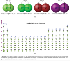
Periodic Trends in Atomic Radii
In each column(group), the atomic radius tends to increase from top to bottom. As you go down the column, the value of “n” for the outermost electrons increases. If the outermost electrons are in larger orbitals, the radius will get larger as there is a greater probability these electrons are further from the nucleus.
Within each row (period), atomic radius tend to decrease from right to left. The reason for this is as you go left to right the orbitals being filled are the same size (for example, going from C to N to O electrons are being added to 2p orbitals), but the nucleus gets more protons, giving it a more positive charge that holds the electrons closer.
Figure 6.30b in OpenStax shows atomic radii pictorially, allowing you to see these trends. There are some exceptions, and the reasoning for these gets complicated (some examples are described in Figure 6.31 and below in OpenStax). In this course, we will concern ourselves with the general trends.
Objective 1 Practice
Ch 7 Objective 2: Predict the relationship between the size of a neutral atom and its ions.
Cations are smaller than their parent atoms.
When a neutral atom loses an electron or electrons to form a cation, there are less electrons to repel each other. Additionally, the electrons removed are typically from the largest orbitals.
Example: A lithium atom (Li) has a radius of 1.34 Å, where Å is an angstrom (1 Å 10-10m). A lithium ion (Li+) is smaller at 0.90 Å.
Anions are larger than their parent atoms.
When neutral atoms add electrons to form anions, the electrons repel each other. The increased electron-electron repulsions cause the electrons to spread out in space, making the radius larger.
Example: A fluorine atom (F) has a radius of 0.71 Å, while a fluoride ion (F–) is larger at 1.19 Å.
For ions carrying the same charge, ion size increases down the group
Similar to what we see in neutral atoms, a higher valence shell (n) means larger orbitals are being filled.
Example: K+ is larger than Na+
Isoelectronic Series
An isoelectronic series is a group of ions all containing the same number of electrons. For example: O2-, F1-,Na+, Mg2+, and Al3+ all have 10 electrons, and all have the same electron configuration as Ne:
Since the number of electrons is constant, the ionic radius decreases with increasing nuclear charge (same number of electrons in same configuration, more positive nucleus).
The radii for our above example are:
| Ion | Radius (Å) |
| O2- | 1.26 |
| F1- | 1.19 |
| Na+ | 1.16 |
| Mg2+ | 0.86 |
| Al3+ | 0.68 |
Objective 1 and 2 Practice
Ch 7 Objective 3: Define ionization energy and electron affinity.
Ch 7 Objective 4: Predict and explain the ionization energies of atoms based on their positions in the periodic table.
Ionization Energy
Ionization energy is the energy required to remove an electron from the ground state of an atom or ion. It is always endothermic. The first ionization energy is for removal of the first electron from the atom. The second ionization energy is for removal of the second electron from the atom (or an electron from the +1 ion).
Equations corresponding to ionization energy
General form for first IE: X → X+ + e–. Notice you start with a neutral atom. removing an electron makes it a product, and the resulting +1 ion is a product as well.
General form for second IE: X+ → X2+ + e–
General Trends in 1st Ionization Energy
The first ionization energy increases from left to right across the period. Why? The nuclear charge increases from left to right, and similar orbitals being filled, so it gets harder to remove an electron.
The first ionization energy increases from bottom to top in a group. Why? The valence electrons are closer to the nucleus as you go up a group.
Therefore, the general periodic trend for first ionization energy is that it increases as you go up and right on the periodic table. Ionization energies for the elements are shown in OpenStax Figure 6.34:
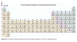
There are some exceptions to this trend, but they are beyond the scope of this course.
General trends for ionization energies beyond the first
It requires more energy to remove each successive electron. Therefore, the second ionization energy is higher than the first, the third is higher than the second, etc. Also, when all valence electrons have been removed, the next ionization energy has a large increase, because removing the next electron takes the ion out of the stable noble gas configuration. This is shown in some of the large jumps in ionization energies in Table 6.3 of OpenStax. The subsection”Variation in Ionization Energies” in Section 6.5 of OpenStax gives an excellent description of these trends in ionization energy and how they connect to electron configuration.
Electron Affinity
Electron affinity is the tendency of an atom to gain an electron to form an anion. The higher the electron affinity, the stronger the tendency to gain an electron. Electron affinity is formally defined as the energy released with the addition of an electron to an atom. A higher electron affinity means the above reaction (addition of an electron) is more exothermic. We can think of it as, “the higher the electron affinity, the more the atom wants to gain an electron to form an ion.”
Equations corresponding to the electron affinity
Notice how these equations are different from those corresponding to ionization energy: the gained electron is a reactant and the element goes from neutral to -1.
General form: X + e– → X–
The general periodic trend for electron affinity is the same as that for ionization energy (increases as go up or right) with the exception of the noble gases, which do not want to gain electrons. Therefore, fluorine has the highest electron affinity.
Electron affinities for the elements are shown in OpenStax Figure 6.35.
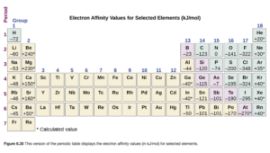
There are some exceptions to this trend, but they are beyond the scope of this course.
Objective 3 and 4 practice
Ch 7 Objective 5: Describe the periodic trends in metallic and nonmetallic character.
In the first unit in this class, you learned that metals tend to lose electrons to form cations, while nonmetals tend to gain electrons to form anions.
Given these definitions, answer the following questions:
Therefore, as you go up and right on the periodic table, elements get more nonmetallic (less metallic character). Elements on the upper right (toward F) have higher electron affinity and tend to form anions, while atoms on the lower left (towards Fr) have lower ionization energies and tend to form cations.
Objective 5 Practice
What’s next?
What you have just learned about the electronic structure of atoms, ions, and elements plays a great role in how elements combine to make compounds and atoms combine to make molecules — that’s what we will look at next.