In CHEM 151, you learned about a theory of chemical bonding called valence bond theory. In this theory, chemical bonds (which contained valence electrons being shared between two bonding atoms) are formed when orbitals from each of the bonding atoms containing each atom’s valence electrons overlap. This theory, along with the concepts of hybridization, Lewis dot structures, and VSEPR, explain many aspects of covalent molecules quite well.
Molecular Orbital Theory uses a different philosophy. The orbitals you learned about in CHEM 151 are called atomic orbitals – as each orbital belongs to the atom. You may recall that an (atomic) orbital is a mathematical equation that is a solution to the Schrodinger Equation that gives a probability density of the location of an electron in an atom. In molecular orbital theory, once atoms are bonded into molecules the orbitals from each atom are no longer valid — instead the molecule has orbitals belonging to the entire molecule. As we will see, molecular orbital theory does explains some aspects of bonding well that valence bond theory does not.
Objective 1:Explain the essential features of the molecular orbital theory.
Valence Bond Theory
This is generally the first theory of bonding students learn about in general chemistry, and was the theory you learned in CHEM 151. According to this theory, covalent bonds result when atoms share outer (valence) electrons. The way atoms share these electrons is the orbitals containing these valence electrons overlap in space. An orbital gives the probability density of location of an electron in an atom. You may recall that each orbital holds two electrons.
Another facet of valence bond theory you may remember is hybridization. Hybrid orbitals are each a mixture of atomic orbitals from a single atom. Many atomic orbitals involved in bonding are hybrid orbitals, and they are oriented to each other in a way that explains the geometries such as tetrahedral, trigonal bipyramidal, etc found in molecules. Hybrid orbitals are still atomic orbitals, though, and remain localized on that atom.
Limitations of Valence Bond Theory
Valence bond theory assumes all bonds are localized bonds in a molecule: for example, in a CH4 molecule, each pair of electrons is confined to the region between the carbon nucleus and the hydrogen nucleus. Also, experimental observations show that some substances (O2 for example) are paramagnetic while others (N2 for example) are diamagetic. Valence bond theory has no explanation for this, but molecular orbital theory does. Valence bond theory also not deal well with odd electron molecules such as NO, but, as we will see, molecular orbital theory does.
Molecular Orbital (MO) Theory
Molecular orbitals (MOs) are linear mathematical combinations of atomic orbitals (AOs) from different atoms. The number of AOs combined is equal to the number of MOs resulting from the combination.
MOs are associated with the entire molecule, not a single atom. However, like an atomic orbital, each MO can hold two electrons of opposite spin.
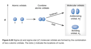
Figure 8.29 in OpenStax shows the combining of two AOs (the s orbitals on the left) to make two MOs (on the right)
Objective 2:Explain the relationship between bonding and antibonding molecular orbitals, both in terms of energy compared to the corresponding atomic orbitals and where electron density is concentrated relative to the nuclei.
There are two general types of molecular orbitals: bonding molecular orbitals and antibonding molecular orbitals. If you look at the figure above, you can see there is one of each.
Bonding MOs
Since atomic orbitals are wave functions, the waves can interact constructively or destructively. In a bonding molecular orbital, the wave functions combine constructively. In a bonding MO, most of the electron density is between adjacent nuclei (see the diagram above). Therefore, bonding MOs are lower in energy that the combined atomic AOs. As a result, they energetically favors bond formation. An electron in a bonding orbital stabilizes a molecule. There are both sigma (σ) and pi (π ) MOs (more on that later).
Antibonding MOs
In an antibonding molecular orbital, the wave functions combine destructively. In these MOs, most of the electron density is not between the nuclei (see the diagram above). In fact, there is a node (a region of zero probability of finding the electrons) between the nuclei. Therefore, bonding MOs are higher in energy than the combined atomic AOs. As a result, they do not favor bond formation. An electron in a bonding orbital destabilizes a molecule. Antibonding MOs are signified by an asterisk *, so you will see σ* and π* antibonding MOs.
Objective 3:Given a molecular orbital diagram for the diatomic molecule or ion built from elements of the first or second period, predict the placement of electrons, the bond order and the number of unpaired electrons. Also, determine whether the molecule is paramagnetic or diamagnetic.
Molecular orbital diagrams
The combination of atomic orbitals and the relative energies of the molecular orbitals are shown by an energy-level (or molecular orbital) diagram. We can think of an MO diagram as a “comparison” diagram – where the atomic orbitals of the individual atoms in the molecule are shown on the same diagram as the molecular orbitals resulting from their combination, allowing for a comparison of energy.
Figure 8.35 in Open Stax shows a MO diagram for the H2 molecule:
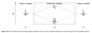
Each hydrogen atom in the molecule has one valence electron (1s1). These are shown on the atomic orbitals (1 for each atom) on the left and right sides of the diagram. The resulting two MOs are shown in the center (note the σ1s bonding MO is lower in energy than the AOs and the σ1s* antibonding MO is higher in energy. The two electrons in the H2 molecule will fill the MOs following the Aufbau principle lowest energy first and Hund’s rules (if you have equal energy orbitals, one electron goes in each first with the same spin before they are filled). Therefore, the two electrons are in the bonding MO.
Calculating Bond Order from MO diagrams
Once the MO diagram is filled, we can calculate the bond order as follows:

A bond order of 1 corresponds to a single bond, 2 a double bond, etc. A bond order 0 means there will be no bonding and that the molecule does not exist.
For H2, the bond order will be:

Next, let’s look at the bond order of He2. He2 has 4 electrons (2 from each He atom)
Figure 8.36 in Open Stax shows a MO diagram for the He2 molecule:
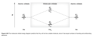
Since the bonding MO is filled with the first two electrons, the second two go into the antibonding. The bond order is:

The bond order of zero means there is no bond between the two He atoms – the He2 molecule does not exist. We could also write a molecular orbital electron configuration for He2:(σ1s)2 (σ*1s)2
MO Diagram Practice
MO Diagrams for Second Row Diatomic Molecules
When we get to the second row of the periodic table, things get more complicated as there are valence 2s and 2p orbitals. As previously seen, though, the same rules still hold:
- The # of MOs formed equals the # of AOs combined
- AOs combine most effectively with other atomic orbitals of similar energy
This means in a diatomic molecule, the two 2s orbitals (one from each atom) will combine to make two MOs (one bonding and one antibonding). The six 2s orbitals (three from each atom) will combine to make six MOs (three bonding and three antibonding).
There is one other complication introduced by the 2p. Combining of 2p AOs yields two types of MOs: sigma (σ) and pi (π ).
Figure 8.30 in OpenStax shows the σ2p MOs (both bonding and antibonding). The MOs are along the internuclear axis.
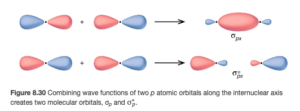
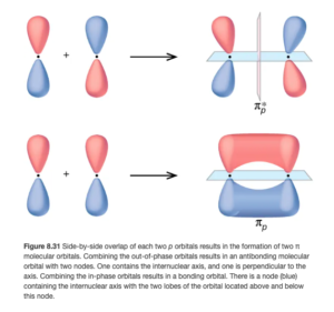
Figure 8.31 in OpenStax shows the π2p MOs (both bonding and antibonding). The MOs are perpendicular the internuclear axis.
What we learned for atomic orbitals still holds: fill the orbitals from low to high energy, half-filling each degenerate (same energy) orbital first before pairing electrons in the same orbital.
Figure 8.37 in OpenStax shows the valence shell MO diagrams for all of the second row elements:
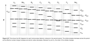
Notice the order or the orbitals change between N2 and O2. In either case, the orbitals will still fill in order of increasing energy.
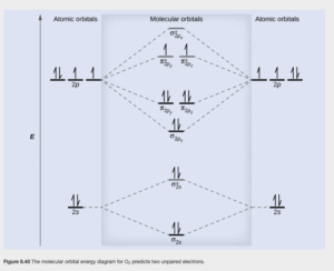
Figure 8.40 (in example 8.6) shows the filled valence orbital diagram for O2. See if you can come up with the same filling using the 12 valence electrons for O2 and the diagram for O2 in Figure 8.37.
OpenStax Table 8.3 shows electron configurations and bond order for the second row diatomics.
Examining the diagram above, we can determine that O2 is paramagmetic. You may remember from the study of coordination chemistry that paramagnetism is indicated if at least one d orbital is half filled with only 1 electron. The same holds true for MOs. Also, if all molecular orbitals are empty or fully filled (no unpaired spins) it is diamagnetic.
MO Diagrams for Second Row Diatomic Molecules- practice
Using Figure 8.37 in OpenStax, fill out the MO diagram for N2 and answer the following questions:
Heteronuclear diatomic molecules
The molecules we have looked at so far are homonuclear diatomic molecules — both atoms are the samre element. MO theory also works well for heteronuclear diatomic molecules such as NO and OF and ions such as CN– or NO+. For example, CN– would have the same filled MO diagram as N2 as they each have 10 valence electrons. You should be able to complete MO diagrams and determine bond order and magnetism for heteronuclear diatomic molecular and diatomic ions as well, including those with an odd number of valence electrons.
Heteronuclear diatomic molecules- practice
Using Figure 8.37 in OpenStax, fill out the MO diagram for CN (you can use the MO diagram for either C2 or N2) and answer the following questions: